
3
CONTINUOUS FUNCTIONS
The definition of "a function is continuous at a value of x"
Limits of continuous functions
CONTINUOUS MOTION is motion that continues without a break. Its prototype is a straight line. There is no limit to the smallness of the distances traversed.
Calculus wants to describe that motion mathematically, both the distance traveled and the speed at any given time, particularly when the speed is not constant. Solving that mathematical problem is one of the first applications of calculus.
In any real problem of continuous motion, the distance traveled will be represented as a "continuous function" of the time traveled because we always treat time as continuous. Therefore, we must investigate what we mean by a continuous function.
A continuous function
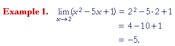
In the previous Lesson, we saw that the limit of a polynomial as x approaches any value c, is simply the value of the polynomial at x = c.
If P(x) is a polynomial, then
![]()
Compare Example 1 and Problem 2 of Lesson 2.
We are about to see that that is the definition of a function being "continuous at the value c." But why?
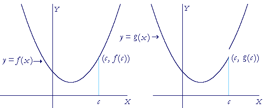
A graph is an aid to seeing a relationship between numbers. Therefore, consider the graph of a function f(x) on the left. That graph is a continuous, unbroken line. Therefore we want to say that f(x) is a continuous function. But a function is a relationship between numbers. (Topic 3 of Precalculus.) Any definition of a continuous function therefore must be expressed in terms of numbers only. To do that, we must see what it is that makes a graph -- a line -- continuous, and try to find that same property in the numbers.
(To avoid scrolling, the figure above is repeated .)
If we think of each graph, f(x) and g(x), as having two branches, two parts -- one to the left of x = c, and the other to the right -- then the graph of f(x) stays connected at x = c. The graph of g(x) on the right does not.
In the graph of f(x), there is no gap between the two parts. Those parts share a common boundary, the point (c, f(c)). We saw in Lesson 1 that
that is what characterizes any continuous quantity. That is why the graph
of f(x) is continuous at x = c.
How can we mathematically define the sentence, "The function f(x) is continuous at x = c."?
Let us think of the values of x being in two parts: one less than x = c, and one greater. Then as x approaches c, both from the left and from the right, if the corresponding values of f(x) -- those numbers -- approach f(c), those values will share a common boundary, namely the one number, f(c). Upon borrowing the word "continuous" from geometry then (Definition 1), we will say that the function is continuous at x = c.
For example, if y = x2, and c = 4, then
![]()
(Lesson 2.)
The limit of x2 as x approaches 4 is equal to 42.
y = x2 is continuous at x = 4.
In the function g(x), however, the limit of g(x) as x approaches c does not exist. If the left-hand limit were the value g(c), the right-hand limit would not be g(c). That function is discontinuous at x = c.
Here is the definition:
DEFINITION 3. A function continuous at a value of x.
We say that a function f(x) that is defined at x = c is continuous at x = c
if the limit of f(x) as x approaches c
is equal to the value of f(x) at x = c.
In symbols, if
![]()
then f(x) is continuous at x = c.
And so for a function to be continuous at x = c, the limit must exist as x approaches c, that is, the left- and right-hand limits -- those numbers -- must be equal. (Definition 2.2)
If a function is continuous at every value in an interval, then we say that the function is continuous in that interval. And if a function is continuous in any interval, then we simply call it a continuous function.
By "every" value, we mean every one we name; any meaning more than that is unnecessary.
Calculus is essentially about functions that are continuous at every value in their domains. Prime examples of continuous functions are polynomials (Lesson 2).
Problem 1.
a) Prove that this polynomial,
f(x) = 2x2 − 3x + 5,
a) is continuous at x = 1.
To see the answer, pass your mouse over the colored area.
To cover the answer again, click "Refresh" ("Reload").
Do the problem yourself first!
We must apply the definition of "continuous at a value of x."
That is, we must show that when x approaches 1 as a limit, f(x) approaches f(1), which is 4.
(According to the theorems on limits, that is true.)
f(x) therefore is continuous at x = 1.
b) Can you think of any value of x where that polynomial -- or any
b) polynomial -- would not be continuous?
You should not be able to. Polynomials are continuous everywhere. As x approaches any limit c, any polynomial
P(x) approaches P(c).
(Lesson 2)
Problems 4, 5, 6 and 7 of Lesson 2 are examples of functions -- polynomials -- that are continuous at each given value.
In addition to polynomials, the following functions also are continuous at every value in their domains.
Rational functions
Root functions
Trigonometric functions
Inverse trigonometric functions
Logarithmic functions
Exponential functions
These are the functions that one encounters throughout calculus.
Limits of continuous functions
Like any definition, the definition of a continuous function is reversible. That means, if
![]()
then we may say that f(x) is continuous. And conversely, if we say that f(x) is continuous, then
![]()
Therefore:
To evaluate the limit of any continuous function as x approaches a value, simply evaluate the function at that value.
![]()
| Example 2. Evaluate |
| Solution. |
The student should have a firm grasp of the basic values of the trigonometric functions. In calculus, they are indispensable. See Topics 15 and 16 of Trigonometry.
| Problem 2. Evaluate |
sin 0 = 0.
| Problem 3. Evaluate |
![]()
Problem 4. Velocity, v(t), is a continuous function of time t. Let
v(t) = 2t 2 + 1.
If distance is measured in meters, and the function is defined at
t = 5 sec, then explain why
![]()
Since v(t) is a continuous function, then the limit as t approaches 5 is equal to the value of v(t) at t = 5.
| * | * | * |
If a function is not continuous at a value, then it is discontinuous at that value. Here is the graph of a function that is discontinuous at x = 0.
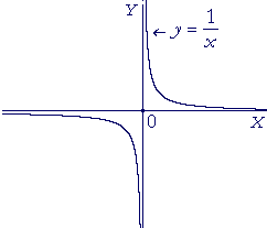
| This is the graph of y = | 1 x |
. At x = 0, the function is not defined, |
because division by 0 is an excluded operation. (Skill in Algebra, Lesson 5.) x = 0 is a point of discontinuity. In fact, as x approaches 0 -- whether from the right or from the left -- y does not approach any number.
Nevertheless, as x increases continuously in an interval that does not include 0, then y will decrease continuously in that interval. We say,
| "The function y = | 1 x |
is continuous for all values of x except x = 0." |
Equivalently,
| "The function y = | 1 x |
is continuous for all values of x in its domain." |
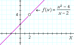
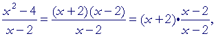
Example 3. Consider this function:
| f(x) | = | x2 − 4 x − 2 |
This function is undefined at x = 2, and therefore it is discontinuous there; however, we will come back to this below.
The function nevertheless is defined at all other values of x, and it is continuous at all other values.
For example, as x approaches 8, then according to the Theorems of Lesson 2, f(x) approaches f(8).
| f(8) = | 60 6 |
= 10. |
f(x) therefore is continuous at x = 8. (Definition 3.)
In this same way, we could show that the function is continuous at all values of x except x = 2.
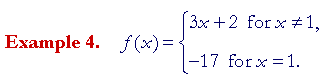
This is an example of a perverse function, in which the function is deliberately assigned a value different from the limit as x approaches 1. That limit is 5. But the value of the function at x = 1 is −17. f(x) is not continuous at x = 1.
In lessons on continuous functions, such problems (logical jokes?) tend to be common. They are constructed to test the student's understanding of the definition of continuity. Such functions have a very brief lifetime however. After the lesson on continuous functions, the student will never see their like again.
For a function to be continuous at x = c, it must exist at x = c. However, when a function does not exist at x = c, it is sometimes possible to assign a value so that it will be continuous there.
This function
| f(x) | = | x2 − 4 x − 2 |
does not exist at x = 2. But for every value of x![]() 2:
2:
| x2 − 4 x − 2 |
= | (x + 2)(x − 2) x − 2 |
= | x + 2. |
Therefore, as x approaches 2,
![]()
(Compare Example 2 of Lesson 2.) That is,
![]()
Now, f(x) is not defined at x = 2 -- but we could define it. We could define it to have the value of that limit![]() We could say,
We could say,
"At x = 2, let f(x) have the value 4."
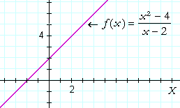
If we do that, then f(x) will be continuous at x = 2 -- because the limit at that value will be the value of the function.
![]()
When we are able to define a function at a value where it is undefined or its value is not the limit, we say that the function has a removable discontinuity.
Note: Since
then upon defining f(2) as 4, then ![]() has effectively been defined as 1.
has effectively been defined as 1.
Problem 5. Consider this function:
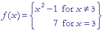
a) For which value of x is this function discontinuous? x = 3.
b) Define the function there so that it will be continuous.
Since the limit of f(x) as x approaches 3 is 8, then if we define f(3) = 8, rather than 7, then we have removed the discontinuity.
![]()
Next Lesson: The "limit" infinity (∞)
Please make a donation to keep TheMathPage online.
Even $1 will help.
Copyright © 2021 Lawrence Spector
Questions or comments?
E-mail: teacher@themathpage.com